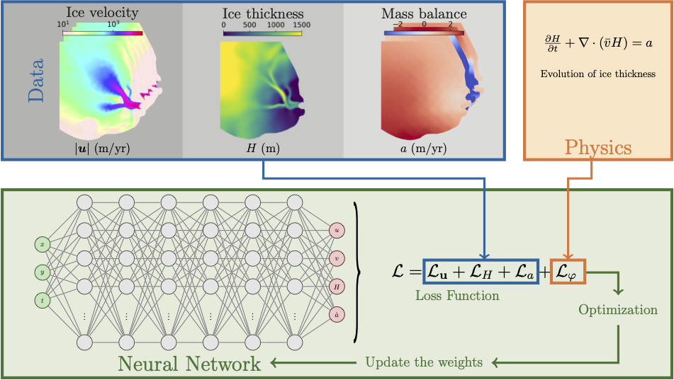
Time-Dependent Forward Modeling of Helheim Glacier

This example demonstrates how to use PINNICLE for solving a time-dependent forward problem, simulating the evolution of ice thickness over time using the mass conservation equation. The case study focuses on Helheim Glacier, Greenland, over the period 2008–2009.

Problem Description

We solve the Mass Conservation The goal is to simulate how ice thickness evolves over time, given velocity and mass balance data as a time series. This is a forward modeling problem with known initial conditions.

\[\frac{\partial H}{\partial t} + \nabla \cdot (\bar{\mathbf{u}} H) = a\]

where:

• \(H\) is ice thickness

• \(\bar{\mathbf{u}} = (u, v)^T\) is the depth-averaged horizontal velocity

• \(a\) is the net surface mass balance

Data and Setup

Data are provided as .mat files (one per time step), derived from a transient ISSM simulation. Each file contains velocity, mass balance, and (for the initial step) thickness.

• Time Range: 2008–2009 (with 11 time steps, every 0.1 years)

• Inputs: \(u\), \(v\), \(a\) at each time step

• Initial condition: \(H\) at \(t = 2008\)

PINNICLE automatically constructs the spatiotemporal domain and trains a network to model \(H(x, y, t)\).

Configuration Snippet

hp["time_dependent"] = True
hp["start_time"] = 2008
hp["end_time"] = 2009
hp["num_layers"] = 6
hp["num_neurons"] = 32
hp["equations"] = {"Mass transport": {}}
hp["shapefile"] = "Helheim_Basin.exp"
hp["num_collocation_points"] = 10000

for t in np.linspace(2008, 2009, 11):
    issm = {}
    if t == 2008:
        issm["data_size"] = {"u":3000, "v":3000, "a":3000, "H":3000}
    else:
        issm["data_size"] = {"u":3000, "v":3000, "a":3000, "H":None}
    issm["data_path"] = f"Helheim_Transient_{t}.mat"
    issm["default_time"] = t
    issm["source"] = "ISSM"
    hp["data"][f"ISSM{t}"] = issm

Loss Function

The total loss includes:

\[L = L_u + L_H + L_a + L_\phi\]

where: - \(L_u\): data misfit for velocity across all time steps - \(L_H\): initial thickness misfit at \(t = 2008\) - \(L_a\): mass balance misfit across time - \(L_\phi\): mass conservation residual at spatiotemporal collocation points

Results

After training for 800,000 epochs, the solution at the initial and final time steps are

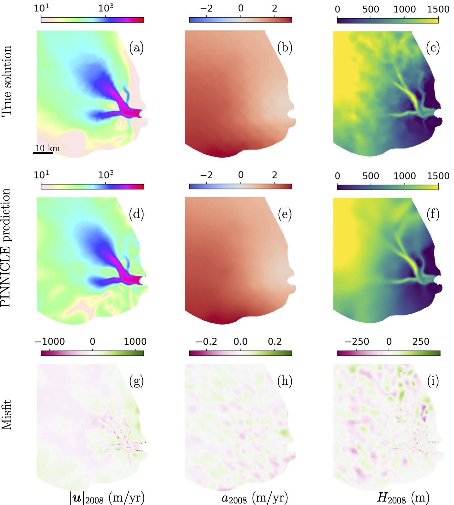
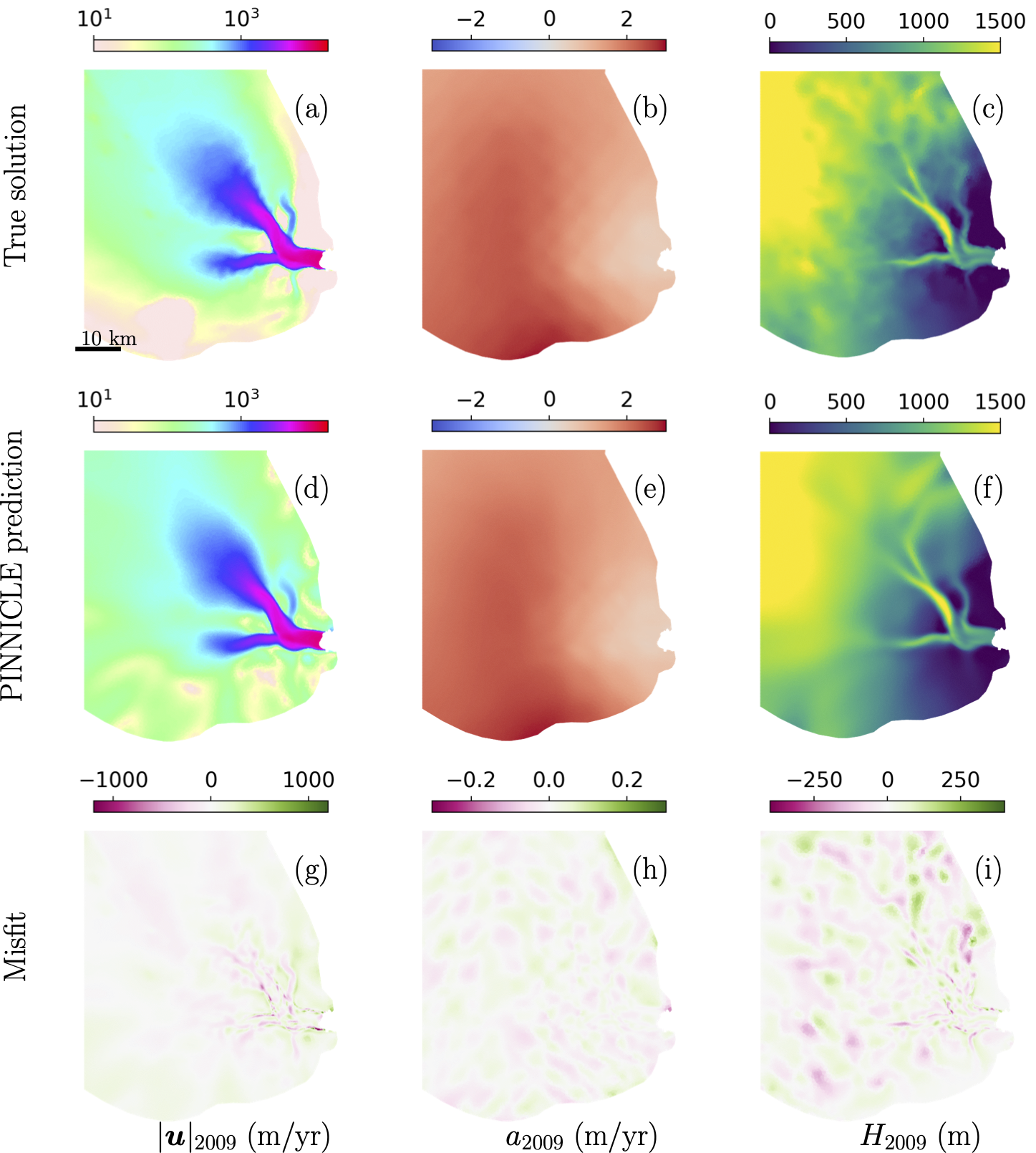
The top rows show the “true” simulation output from ISSM, the middle rows show PINNICLE predictions, and the bottom rows show misfits.

References

• Cheng et al. (2022). “Helheim Glacier’s Terminus Position Controls Its Seasonal and Inter-Annual Ice Flow Variability”

• Cheng et al. (2024). “Forward and Inverse Modeling of Ice Sheet Flow Using Physics-Informed Neural Networks”

Complete code

import pinnicle
import numpy as np

# hyperparameters
hp = {}
hp["epochs"] = 800000

# time dependent problem
hp["time_dependent"] = True
hp["start_time"]     = 2008
hp["end_time"]       = 2009

# NN
hp["num_neurons"] = 32
hp["num_layers"]  = 6

# domain
hp["shapefile"] = "Helheim_Basin.exp"
hp["num_collocation_points"] = 10000

# physics
hp["equations"] = {"Mass transport":{}}

# data
hp["data"] = {}
for t in np.linspace(2008,2009,11):
    issm = {}
    if t == 2008:
        issm["data_size"] = {"u":3000, "v":3000, "a":3000, "H":3000}
    else:
        issm["data_size"] = {"u":3000, "v":3000, "a":3000, "H":None}
        
    issm["data_path"]         = "Helheim_Transient_" + "%g"%t + ".mat"
    issm["default_time"]      = t
    issm["source"]            = "ISSM"
    hp["data"]["ISSM"+"%g"%t] = issm

# create experiment
experiment = pinnicle.PINN(hp)
experiment.compile()

# Train
experiment.train()