Inverse Problem on Helheim Glacier
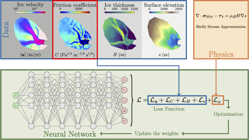
This example illustrates PINNICLE’s ability to solve a classical inverse problem in glaciology: inferring the basal friction coefficient from surface observations using the Shelfy-Stream Approximation (SSA) model.
The case study is based on Helheim Glacier, located in Southeast Greenland.
Problem Description
The task is to infer the spatially varying basal friction coefficient \(C(x, y)\) by minimizing the misfit between model and observed ice surface velocity (\(u\), \(v\)) The governing equations are the SSA momentum balance equations, with basal friction modeled by Weertman’s law:
Configuration
The problem is configured using:
hp["epochs"] = 100000
hp["num_layers"] = 6
hp["num_neurons"] = 20
hp["shapefile"] = "Helheim.exp"
hp["num_collocation_points"] = 9000
hp["equations"] = {"SSA": {}}
Data is provided from an ISSM model output in Helheim.mat:
issm = {
    "data_path": "Helheim.mat",
    "data_size": {"u": 4000, "v": 4000, "s": 4000, "H": 4000, "C": None}
}
hp["data"] = {"ISSM": issm}
Setting "C": None means that basal friction should be treated as an Dirichlet boundary condition and the interior is inferred by PINNICLE.
Indeed, if the keyword "C" is not even mentioned in "data_size", then it will be treated as an unknown, and inferred completely by PINNICLE.
Loss Function
The total loss includes:
where: - \(L_u\): misfit of velocity (x and y components) - \(L_H\): misfit of ice thickness - \(L_s\): misfit of surface elevation - \(L_C\): Dirichlet boundary condition constraint on \(C\) - \(L_\phi\): residual of the SSA equations (physical loss)
Each term is weighted appropriately using PINNICLE’s default weights.
Results
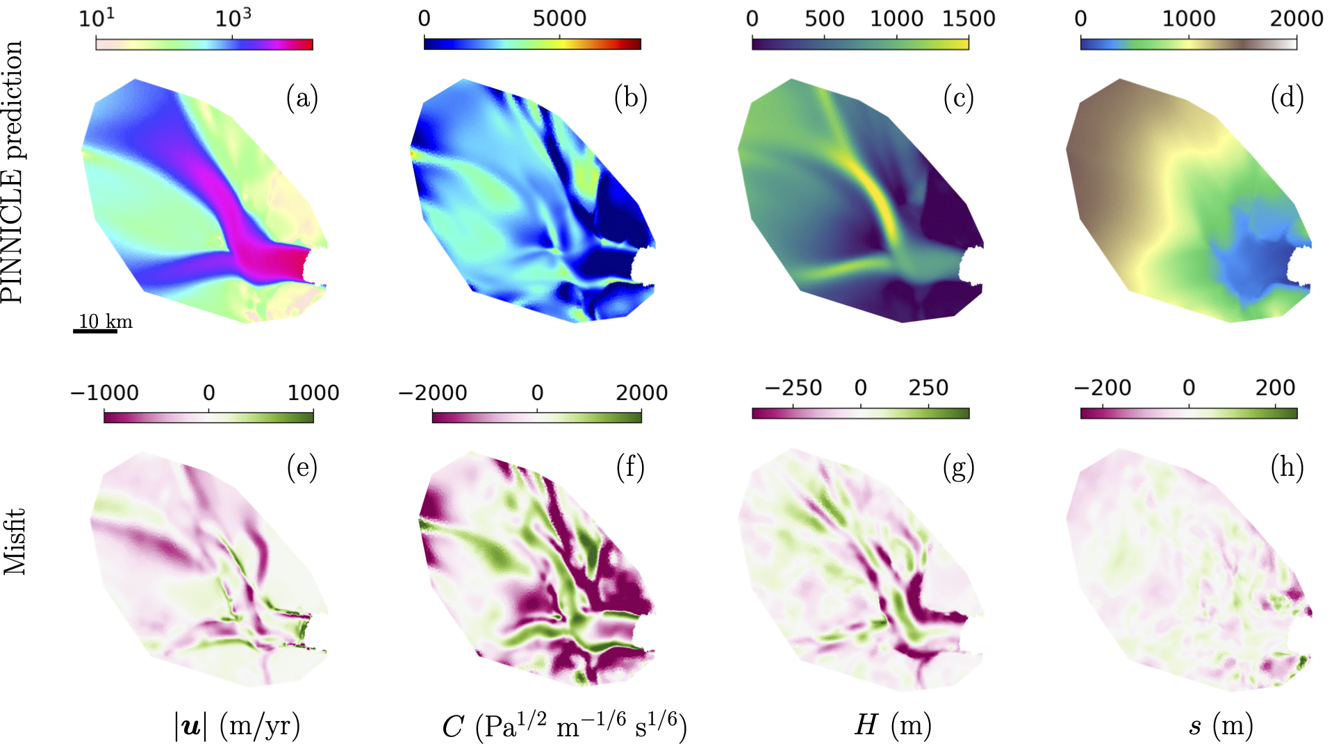
First row: PINNICLE predictions
Second row: misfit compared to the data and eference solution
References
Cheng et al. (2024). “Forward and Inverse Modeling of Ice Sheet Flow Using Physics-Informed Neural Networks”
MacAyeal, D. R. (1989). “Large-scale ice flow over a viscous basal sediment”
Weertman, J. (1957). “On the sliding of glaciers”
Complete code
import pinnicle

# General parameters
hp = {}
hp["epochs"] = 100000

# NN
hp["num_neurons"] = 20
hp["num_layers"] = 6

# domain
hp["shapefile"] = "Helheim.exp"
hp["num_collocation_points"] = 9000

# physics
hp["equations"] = {"SSA":{}}

# data
issm = {}
issm["data_size"] = {"u":4000, "v":4000, "s":4000, "H":4000, "C":None}
issm["data_path"] = "Helheim.mat"
hp["data"] = {"ISSM":issm}

# create experiment
experiment = pinnicle.PINN(hp)
experiment.compile()

# Train
experiment.train()