Simultaneous Inference of Basal Friction and Ice Rheology

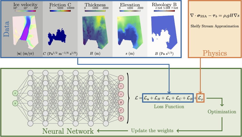
This example showcases PINNICLE’s ability to solve multi-parameter inverse problems, where both basal friction and ice rheology are simultaneously inferred from observational data, using the Shelfy-Stream Approximation (SSA) model. The case study uses real geometry from Pine Island Glacier (PIG), Antarctica.

Problem Description

The goal is to infer two spatially varying parameters:

• Basal friction coefficient (\(C\)) beneath grounded ice

• Rheology pre-factor (\(B\)) within the floating ice shelf

The problem is solved using the SSA with Glen’s flow law, expressed as:

\[\nabla \cdot \sigma_{\text{SSA}} - \tau_b = \rho_i g H \nabla s\]

with:

• \(\sigma_{\text{SSA}}\): stress tensor

• \(\tau_b = C^2 |\mathbf{u}|^m\): basal friction (Weertman law)

The stress tensor is defined as

\[\begin{split}\sigma_{\text{SSA}} = \mu H\begin{bmatrix} 4 \frac{\partial u}{\partial x} + 2\frac{\partial v}{\partial y} & \frac{\partial u}{\partial y} + \frac{\partial v}{\partial x} \\ \frac{\partial u}{\partial y} + \frac{\partial v}{\partial x} & 2\frac{\partial u}{\partial x} + 4\frac{\partial v}{\partial y} \end{bmatrix}\end{split}\]

where the viscosity \(\mu\) is

\[\mu = \frac{B}{2} \left[ \left( \frac{\partial u}{\partial x} \right)^2 + \left( \frac{\partial v}{\partial y} \right)^2 + \frac{1}{4} \left( \frac{\partial u}{\partial y} + \frac{\partial v}{\partial x} \right)^2 + \frac{\partial u}{\partial x} \frac{\partial v}{\partial y} \right]^{\frac{1-n}{2n}}\]

where \(B\) is a spatially varying pre-factor.

Configuration

The domain is larger than the examples of Helheim Glacier and uses more data and collocation points to ensure adequate resolution. We use "SSA_VB" equation to account for spatial dependent pre-factor \(B\).

hp["epochs"] = 1000000
hp["num_layers"] = 6
hp["num_neurons"] = 40
hp["fft"] = True
hp["sigma"] = 10
hp["num_fourier_feature"] = 30
hp["shapefile"] = "PIG.exp"
hp["num_collocation_points"] = 18000
hp["equations"] = {"SSA_VB": {}}

We also need to set, as boundary conditions, for the pre-factor \(B\) to constant \(1.41 \times 10^8 \ \text{Pa s}^{1/3}\) on the grounded ice and friction coefficient \(C=0\) for the floating ice:

hp["data"] = {
    "ISSM": {
        "data_path": "PIG.mat",
        "data_size": {"u": 8000, "v": 8000, "s": 8000, "H": 8000}
    },
    "BC": {
        "data_path": "BC.mat",
        "data_size": {"C": 4000, "B": 4000},
        "source": "mat"
    }
}

Loss Function

The total loss includes:

\[L = L_u + L_H + L_s + L_C + L_B + L_\phi\]

where:

• \(L_u, L_H, L_s\): data misfit terms for velocity, thickness, surface elevation

• \(L_C, L_B\): boundary condition for basal friction and rheology

• \(L_\phi\): PDE residual from SSA equations

Results

After 1,000,000 epochs, PINNICLE infers the following:

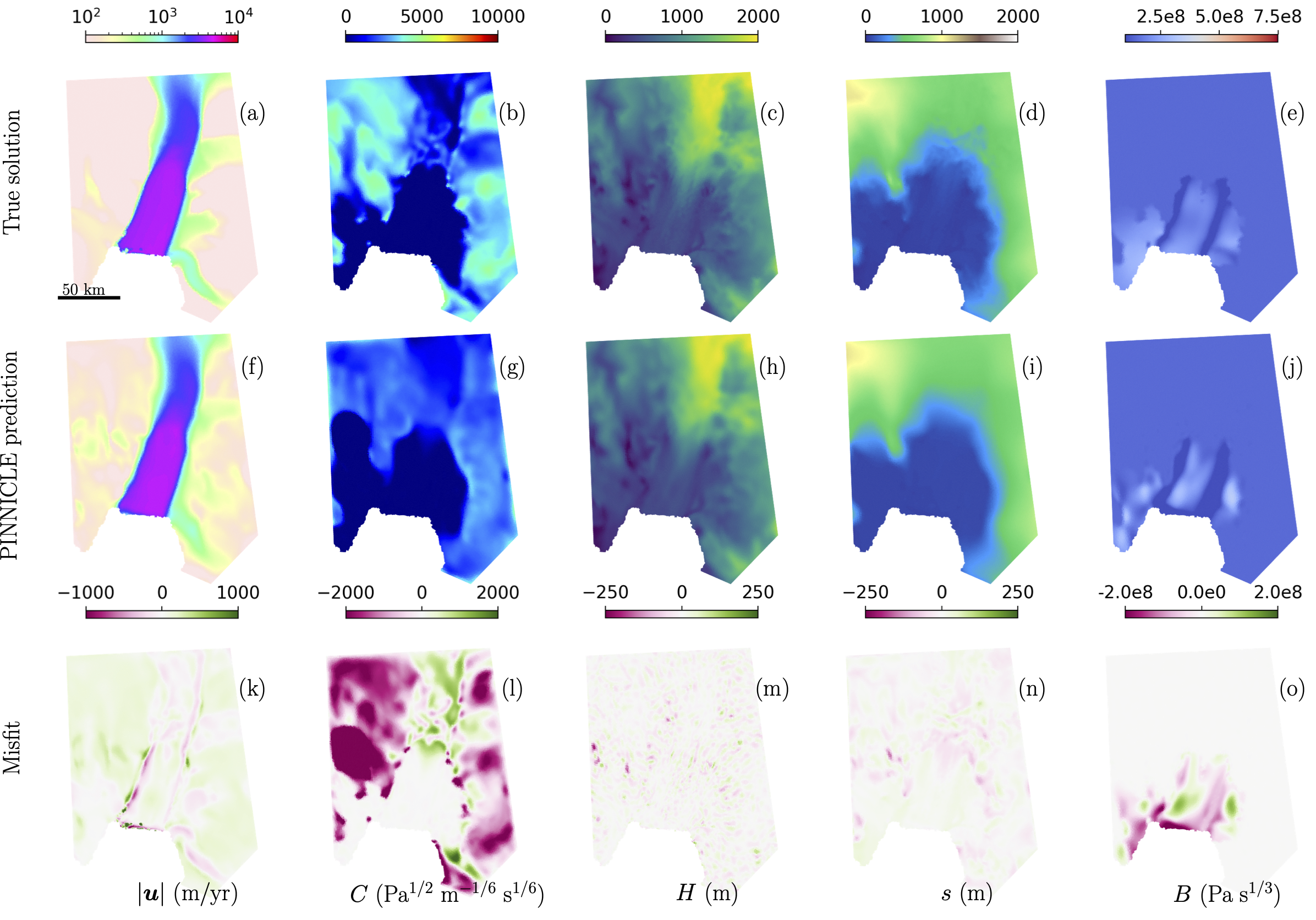
• First row: reference “true solution” (from ISSM)

• Second row: PINNICLE predictions

• Third row: misfit between prediction and reference

References

• Cheng et al. (2024). “Forward and Inverse Modeling of Ice Sheet Flow Using Physics-Informed Neural Networks”

Complete code

import pinnicle

# hyperparameters
hp = {}
hp["epochs"] = 1000000

# NN
hp["num_neurons"] = 40
hp["num_layers"]  = 6
hp["fft"] = True
hp['sigma'] = 10
hp['num_fourier_feature'] = 30

# domain
hp["shapefile"] = "PIG.exp"
hp["num_collocation_points"] = 18000

# physics
hp["equations"] = {"SSA_VB": {}}

# data
issm = {}
issm["data_size"] = {"u":8000, "v":8000, "s":8000, "H":8000}
issm["data_path"] = "PIG.mat"
B = {"data_size":{"B":4000}, "data_path":"B.mat", "source":"mat"}
C = {"data_size":{"C":4000}, "data_path":"C.mat", "source":"mat"}

hp["data"] = {"ISSM":issm, "B":B, "C":C}

# create experiment
experiment = pinnicle.PINN(hp)
experiment.compile()

# Train
experiment.train()